1 Prepare Ticks data

The tick data is user generated with the TickApp, see Section 1 .

library("dplyr")
library("sf")
library("readr")
library("ggplot2")
library("plotly")
library("purrr")
library("janitor")
library("lubridate")

options("sf_max.plot" = 1)

tick_reports <- read_csv("data-raw/classified/tick-reports.csv")

Rows: 68375 Columns: 17
── Column specification ────────────────────────────────────────────────────────
Delimiter: ","
chr  (3): date, uuid, comment
dbl (14): ID, Lat., Lon., x, y, acc., date acc., body part, report type, age...

ℹ Use `spec()` to retrieve the full column specification for this data.
ℹ Specify the column types or set `show_col_types = FALSE` to quiet this message.

swissboundaries_path <- "data-raw/public/swissTLM/swissBOUNDARIES3D_1_4_LV95_LN02.gdb"
# st_layers(swissboundaries_path)

switzerland <- read_sf(swissboundaries_path, "TLM_LANDESGEBIET") |>
  st_zm() |>
  filter(NAME != "Liechtenstein") |>
  st_union() |>
  st_transform(2056)

# clean column names and format columns
tick_reports <- tick_reports |>
  janitor::clean_names() |>
  mutate(across(c(id, x, y, acc, body_part, report_type, age, gender, host, pickup, deleted), ~ as.integer(.x))) |>
  mutate(across(c(lat, lon, date_acc), ~ as.numeric(.x))) |>
  mutate(
    datetime = as.POSIXct(date, format = "%Y-%m-%d %H:%M:%S"),
    date = as.Date(datetime)
  )

# remove rows without a data or data is older than 2015
tick_reports <- tick_reports |>
  filter(!is.na(date)) |>
  filter(date > "2015-01-01")



# remove reports outside a oversized bounding box
# This is redundant, as the data will be filtered by swissBOUNDARIES3D later
XMIN_21781 <- 485000
XMAX_21781 <- 834000
YMAX_21781 <- 296000
YMIN_21781 <- 075000

tick_reports <- tick_reports %>%
  filter(x < XMAX_21781, x > XMIN_21781) %>%
  filter(y < YMAX_21781, y > YMIN_21781)

# remove reports without a uuid or reports that are marked as deleted
tick_reports <- tick_reports %>%
  filter(uuid != "") %>%
  filter(deleted != 1)


# till now, all steps are relatively straightforward. Now, opinions start to
# matter.

# remove reports with a spatial accuracy of more than 1 km radius
tick_reports <- tick_reports |>
  filter(acc < 1000)

# this step is not necessary anymore, I'll keep it here to document
# default acc values. There are more default values it seems, as can be seen
# when visualizing the data as a histogram
tick_reports <- tick_reports %>%
  filter(!(acc %in% c(57274L, 64434L, 1014L)))

tick_reports_sf <- st_as_sf(tick_reports, coords = c("lon", "lat"), crs = 4326)

# I dont know who came up with this, but it doesn't seem to be the case that there
# are more locations near the default locations than outside
default_locations <- data.frame(lat = c(47.3647, 46.81), lon = c(8.5534, 8.23)) |>
  st_as_sf(coords = c("lon", "lat"), crs = 4326)

is_default <- st_is_within_distance(tick_reports_sf, default_locations, 1000) |>
  map_lgl(\(x)length(x) > 0)

sum(is_default)

[1] 23

# date accuracy only has two values: 43'200 and 432'000 (0.5 and 5 days?)
# There are only 8k reports for the higher value, we can discard these
table(tick_reports$date_acc)


 43200 432000 
 39959   8253

tick_reports <- tick_reports |>
  filter(date_acc < 50000)

tick_reports$date_acc <- NULL
tick_reports$body_part <- NULL
tick_reports$report_type <- NULL
tick_reports$age <- NULL
tick_reports$gender <- NULL
tick_reports$host <- NULL
tick_reports$pickup <- NULL
tick_reports$uuid <- NULL
tick_reports$comment <- NULL
tick_reports$deleted <- NULL

# some reports are obivously duplicates: same x and y and date (time may vary slighly)
tick_reports |>
  group_by(x, y, date) |>
  filter(n() > 1) |>
  select(id, datetime)

Adding missing grouping variables: `x`, `y`, `date`

# A tibble: 397 × 5
# Groups:   x, y, date [176]
        x      y date          id datetime           
    <int>  <int> <date>     <int> <dttm>             
 1 609729 261433 2015-04-13   118 2015-04-13 08:34:29
 2 609729 261433 2015-04-13   119 2015-04-13 08:34:29
 3 731962 253501 2015-08-26  2028 2015-08-26 20:46:02
 4 731962 253501 2015-08-26  2029 2015-08-26 20:46:02
 5 621424 264799 2016-07-18  5737 2016-07-18 13:52:11
 6 621424 264799 2016-07-18  5738 2016-07-18 13:53:07
 7 634791 249092 2016-07-25  5967 2016-07-25 08:18:49
 8 634791 249092 2016-07-25  5968 2016-07-25 08:18:49
 9 634791 249092 2016-07-25  5969 2016-07-25 08:18:49
10 667235 212674 2016-08-04  6233 2016-08-04 09:34:30
# ℹ 387 more rows

# keep only distinct reports
tick_reports <- tick_reports |>
  distinct(x, y, date, .keep_all = TRUE)


tick_reports$x <- NULL
tick_reports$y <- NULL

tick_reports_sf <- st_as_sf(tick_reports, coords = c("lon", "lat"), crs = 4326) |>
  st_transform(2056)


tick_reports_sf <- cbind(tick_reports_sf, st_coordinates(tick_reports_sf))

tick_reports_sf <- tick_reports_sf[switzerland, , ]


tick_reports_sf$year <- year(tick_reports_sf$date)

ggplot(tick_reports_sf) +
  geom_sf() +
  facet_wrap(~year)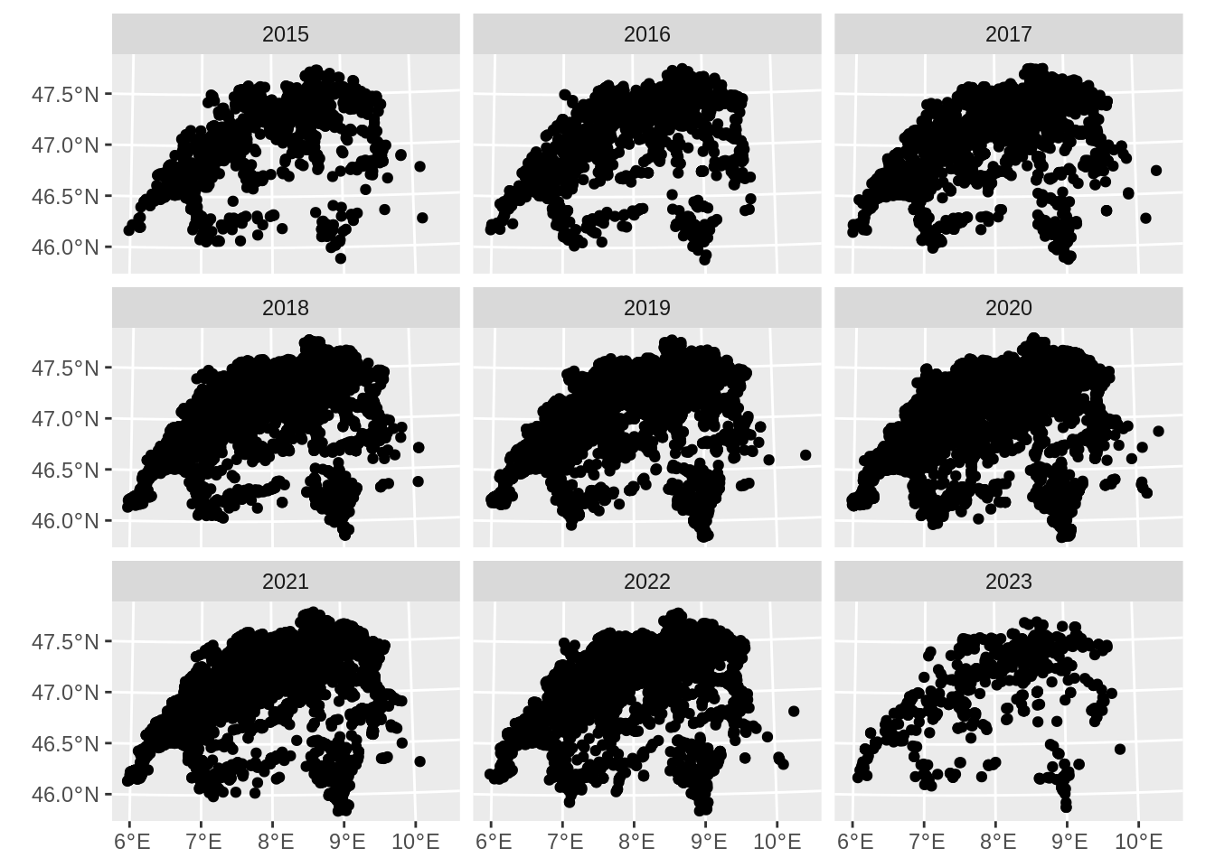

tick_reports_sf$year <- NULL

ticks_path <- "data-processed/Ticks"

if(!dir.exists(ticks_path)) {dir.create(ticks_path)}

st_write(tick_reports_sf, file.path(ticks_path, "tick_reports.gpkg"), "reports_0.1", overwrite = TRUE)

Layer reports_0.1 in dataset data-processed/Ticks/tick_reports.gpkg already exists:
use either append=TRUE to append to layer or append=FALSE to overwrite layer

Error in eval(expr, envir, enclos): Dataset already exists.